Unsupervised Machine Learning: Flat Clustering

K-Means clusternig example with Python and Scikit-learn

This series is concerning "unsupervised machine learning." The difference between supervised and unsupervised machine learning is whether or not we, the scientist, are providing the machine with labeled data.

Unsupervised machine learning is where the scientist does not provide the machine with labeled data, and the machine is expected to derive structure from the data all on its own.

There are many forms of this, though the main form of unsupervised machine learning is clustering. Within clustering, you have "flat" clustering or "hierarchical" clustering.

Now, what can we use unsupervised machine learning for? In general, unsupervised machine learning can actually solve the exact same problems as supervised machine learning, though it may not be as efficient or accurate.

Unsupervised machine learning is most often applied to questions of underlying structure. Genomics, for example, is an area where we do not truly understand the underlying structure. Thus, we use unsupervised machine learning to help us figure out the structure.

Unsupervised learning can also aid in "feature reduction." A term we will cover eventually here is "Principal Component Analysis," or PCA, which is another form of feature reduction, used frequently with unsupervised machine learning. PCA attempts to locate linearly uncorrelated variables, calling these the Principal Components, since these are the more "unique" elements that differentiate or describe whatever the object of analysis is.

There is also a meshing of supervised and unsupervised machine learning, often called semi-supervised machine learning. You will often find things get more complicated with real world examples. You may find, for example, that first you want to use unsupervised machine learning for feature reduction, then you will shift to supervised machine learning once you have used, for example, Flat Clustering to group your data into two clusters, which are now going to be your two labels for supervised learning.

What might be an actual example of this? How about we're trying to differentiate between male and female faces. We aren't already sure what the defining differences between a male and female face are, so we take to unsupervised machine learning first. Our hopeful goal will be to create an algorithm that will naturally just group the faces into two groups. We're likely to go ahead and use Flat Clustering for this, and then we'll likely test the algorithm to see if it was indeed accurate, using labeled data only for testing, not for training. If we find the machine is successful, we now actually have our labels, and features that make up a male face and a female face. We can then use PCA, or maybe we already did. Either way, we can try to get feature count down. Once we've done this, we use these labels with their Principle Components as features, which we can then feed into a supervised machine learning algorithm for actual future identification.

Now that you know some of the uses and some key terms, let's see an actual example with Python and the Scikit-learn (sklearn) module.

import numpy as np
import matplotlib.pyplot as plt
from matplotlib import style
style.use("ggplot")
from sklearn.cluster import KMeans
		

The KMeans import from sklearn.cluster is in reference to the K-Means clustering algorithm. The general idea of clustering is to cluster data points together using various methods. You can probably guess that K-Means uses something to do with means. What ends up happening is a centroid, or prototype point, is identified, and data points are "clustered" into their groups by the centroid they are the closest to.

One of the things that makes any new topic confusing is a lot of complex sounding terms. I do my best to keep things simple, but not everyone is as kind as me.

Some people will refer to the style of clusters that you wind up seeing as "Voronoi" cells. Usually the "clusters" have defining "edges" to them that, when shaded or colored in, look like geometrical polygons, or cells, like this:

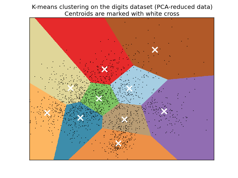
The K-Means algorithm gets its origins from "Lloyd's Algorithm," which basically does the exact same thing.

x = [1, 5, 1.5, 8, 1, 9]
y = [2, 8, 1.8, 8, 0.6, 11]

plt.scatter(x,y)
plt.show()
		

Running the code up to this point will provide you with the following graph:

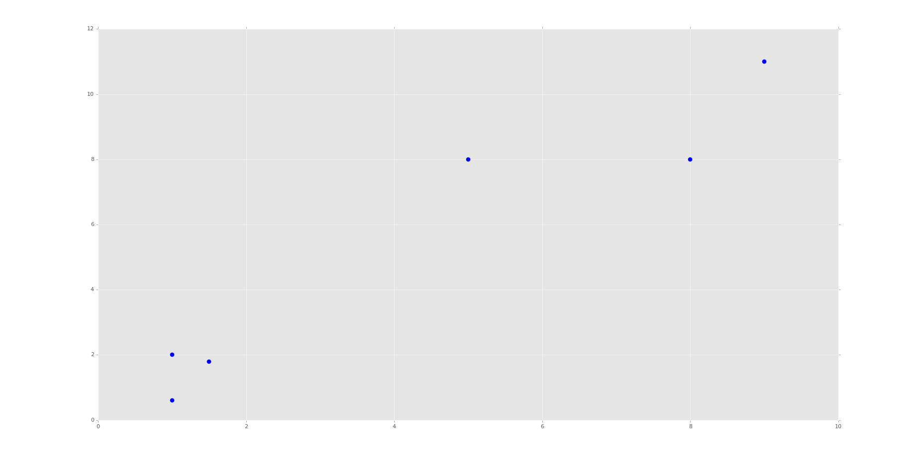
This is the same set of data and graph that we used for our Support Vector Machine / Linear SVC example with supervised machine learning.

You can probably look at this graph, and group this data all on your own. Imagine if this graph was 3D. It would be a little harder. Now imagine this graph is 50-dimensional. Suddenly you're immobilized!

In the supervised machine learning example with this data, we were allowed to feed this data to the machine along with labels. Thus, the lower left group had labeling, and the upper right grouping did too. Our task there was to then accept future points and properly group them according the groups. Easy enough.

Our task here, however, is a bit different. We do not have labeled data, and we want the machine to figure out all on its own that it needs to group the data.

For now, since we're doing flat-clustering, our task is a bit easier since we can tell the machine that we want it categorized into two groups. Still, however, how might you do this?

K-Means approaches the problem by finding similar means, repeatedly trying to find centroids that match with the least variance in groups

This repeatedly trying ends up leaving this algorithm with fairly poor performance, though performance is an issue with all machine learning algorithms. This is why it is usually suggested that you use a highly stream-lined and efficient algorithm that is already tested heavily rather than creating your own.

You also have to decide, as the scientist, how highly you value precision as compared to speed. There is always a balance between precision and speed/performance. More on this later, however. Moving on with the code

X = np.array([[1, 2],
              [5, 8],
              [1.5, 1.8],
              [8, 8],
              [1, 0.6],
              [9, 11]])
		

kmeans = KMeans(n_clusters=2)
kmeans.fit(X)

centroids = kmeans.cluster_centers_
labels = kmeans.labels_

print(centroids)
print(labels)
		

Note here that the "labels" here are labels that the machine has assigned on its own, same with the centroids.

Now we're going to actually plot and visualize the machine's findings based on our data, and the fitment according to the number of clusters we said to find.

colors = ["g.","r.","c.","y."]

for i in range(len(X)):
    print("coordinate:",X[i], "label:", labels[i])
    plt.plot(X[i][0], X[i][1], colors[labels[i]], markersize = 10)


plt.scatter(centroids[:, 0],centroids[:, 1], marker = "x", s=150, linewidths = 5, zorder = 10)

plt.show()
		

The above code is all "visualization" code, having nothing more to do with Machine Learning than just showing us some results.

First, we have a "colors" list. This list will be used to be iterated through to get some custom colors for the resulting graph. Just a nice box of colors to use.

We only need two colors at first, but soon we're going to ask the machine to classify into other numbers of groups just for learning purposes, so I decided to put four choices here. The period after the letters is just the type of "plot marker" to use.

Now, we're using a for loop to iterate through our plots.

If you're confused about the actual code being used, especially with iterating through this loop, or the scatter plotting code slices that look like this: [:, 0], then check out the video. I explain them there.

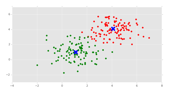
The resulting graph, after the one that just shows the points, should look like:

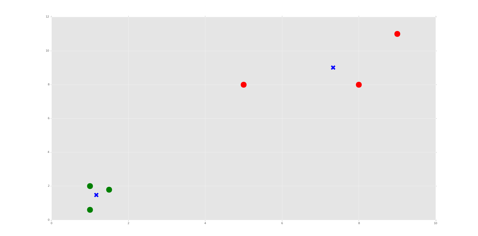
Do you see the Voronoi cells? I hope not, we didn't draw them. Remember, those are the polygons that mark the divisions between clusters. Here, we have each plot marked, by color, what group it belongs to. We have also marked the centroids as big blue "x" shapes.

As we can see, the machine was very successful! Now, I encourage you to play with the n_clusters variable. First, decide how many clusters you will do, then try to predict where the centroids will be.

We do this in the video, choosing 3 and 4 clusters. It's relatively easy to predict with these points if you understand how the algorithm works, and makes for a good learning exercise.

That's it for our Flat Clustering example for unsupervised learning, how about Hierarchical Clustering next?

The next tutorial: Unsupervised Machine Learning: Hierarchical Clustering