Reinforcement Learning in Python with Stable Baselines 3
Welcome to a tutorial series covering how to do reinforcement learning with the Stable Baselines 3 (SB3) package. The objective of the SB3 library is to be for reinforcement learning like what sklearn is for general machine learning. I personally recently embarked on a reinforcement learning challenge with robot dogs, and was finding it quite challenging to iterate through various reinforcement learning algorithms and structures. Stable Baselines 3 enables you to try things like PPO, then maybe some TD3 and then why not try some SAC?!
I had been manually setting things up every time, and this was obviously tedious as well as error-prone. SB3 is almost too easy to use, such that you could probably use it with some mediocre success without any knowledge of reinforcement learning. I will do my best to give some quick basics before diving in, but this is very much going to be a practical and applied tutorial, rather than breaking down each of these algorithms. The SB3 website also contains links and resources to the original papers for algorithms and even some followup information in many cases. There's really no need for you to know every single RL algorithm, just to try them, and I think it's completely reasonable to try some algorithms on some problem, then do more research into the ones that seem promising to you. To start, here are some quick words and definitions that you're likely to come across:
- The Environment: What are you trying to solve? (cartpole, lunar lander, some other custom environment). If you're trying to make some AI play a game, the game is the environment.
- The Model: What algorithm are you using (PPO, SAC, TRPO, TD3...etc).
- The Agent: this is the thing that interacts with the environment using an algorithm/model.
Then, looking closer at the environments, you have two major elements:
- The Observation (or "state"): What is the state of the environment? This could be imagery/visuals, or just vector information. For example, your observation in cartpole is the angle and velocity of the pole. In the bipedal walker environment, the observation contains readings from lidar, the hull's angle, leg positions...etc. An observation is all of this information at some point in time. The observation space is a description, mainly the shape, of those observations.
- The Action: What are the options for your agent in this environment? For example, in cartpole, you can either push left or right. The action space is a description of these possible actions, both in terms of the shape and type (discrete or continuous).
- Step: Take a step in the environment. In general, you pass your action to the step method, the environment performs the step and returns a new observation and reward. You can think of this like frames per second. If you're playing 30 frames per second, then you could have 30 steps per second, but it can get far more complicated than this. A step is just simply progressing in the environment.
What's discrete and continuous?
- Discrete: Think of discrete like classifications. Cartpole has a discrete actionspace. You can go left, or right. Nothing in between, there's no concept of sort of left or half left. It's left, or right.
- Continuous: Think of continuous like regression. It's a range of nearly infinite possibilities. The bidpedal walker environement is a continuous action space, because you set the servo torque anywhere in a range between -1 and positive 1.
Typically, a continuous environment is harder to learn, but sometimes this is a requirement. In robotics, servos/motors of decent quality tend to be naturally largely continuous. Even servos, however, are *actually* discrete, with something like 32,768 positions, but this large of a discrete space is, typically, far too big for a discrete space. That said, there are ways to convert continuous spaces to discrete, in effort to make training faster and easier, and maybe more on that later on. For now, it's just important to understand the two major types of action spaces, as well as the general description of environments, agents, and models.
Once you find some algorithm that seems to be maybe working and learning something, you should dive more deeply into that model, how it works, and the various hyperparameter options that you can tweak.
With all of that out of the way, let's play! To start, you will need Pytorch and stable-baselines3. For Pytorch, just follow the instructions here: Pytorch getting started. For stable-baselines3: pip3 install stable-baselines3[extra]. Finally, we'll need some environments to learn on, for this we'll use Open AI gym, which you can get with pip3 install gym[box2d]. On linux for gym and the box2d environments, I also needed to do the following:
		apt install xvfb ffmpeg xorg-dev libsdl2-dev swig cmake
		pip3 install gym[box2d]
For this tutorial, I'll start us off with the lunar lander environment. Later I will cover how you can use your own custom environment too. First, let's get a grasp of the fundamentals of our environment. When choosing algorithms to try, or creating your own environment, you will need to start thinking in terms of observations and actions, per step. While your own custom RL problems are probably not coming from OpenAI's gym, the structure of an OpenAI gym problem is the standard by which basically everyone does reinforcement learning. Let's take a peak at the lunar lander environment:
import gym

# Create the environment
env = gym.make('LunarLander-v2')  # continuous: LunarLanderContinuous-v2

# required before you can step the environment
env.reset()

# sample action:
print("sample action:", env.action_space.sample())

# observation space shape:
print("observation space shape:", env.observation_space.shape)

# sample observation:
print("sample observation:", env.observation_space.sample())

env.close()
Running that, you should see something like:
sample action: 2
observation space shape: (8,)
sample observation: [-0.51052296  0.00194223  1.4957197  -0.3037317  -0.20905018 -0.1737924
	1.8414629   0.09498857]
Our actions are discrete, and just 1 discrete action of 0, 1, 2, or 3. 0 means do nothing, 1 means fire the left engine, 2 means fire the bottom engine, and 3 means fire the right engine. The observation space is a vector of 8 values. Looking at the gym code for this environment, we can find out what the values in the observation mean https://github.com/openai/gym/blob/master/gym/envs/box2d/lunar_lander.py#L447:
        env: The environment
	s (list): The state. Attributes:
				s[0] is the horizontal coordinate
				s[1] is the vertical coordinate
				s[2] is the horizontal speed
				s[3] is the vertical speed
				s[4] is the angle
				s[5] is the angular speed
				s[6] 1 if first leg has contact, else 0
				s[7] 1 if second leg has contact, else 0
We can see a sample of the environment by running:
import gym


env = gym.make('LunarLander-v2')  # continuous: LunarLanderContinuous-v2
env.reset()

for step in range(200):
	env.render()
	# take random action
	env.step(env.action_space.sample())

env.close()

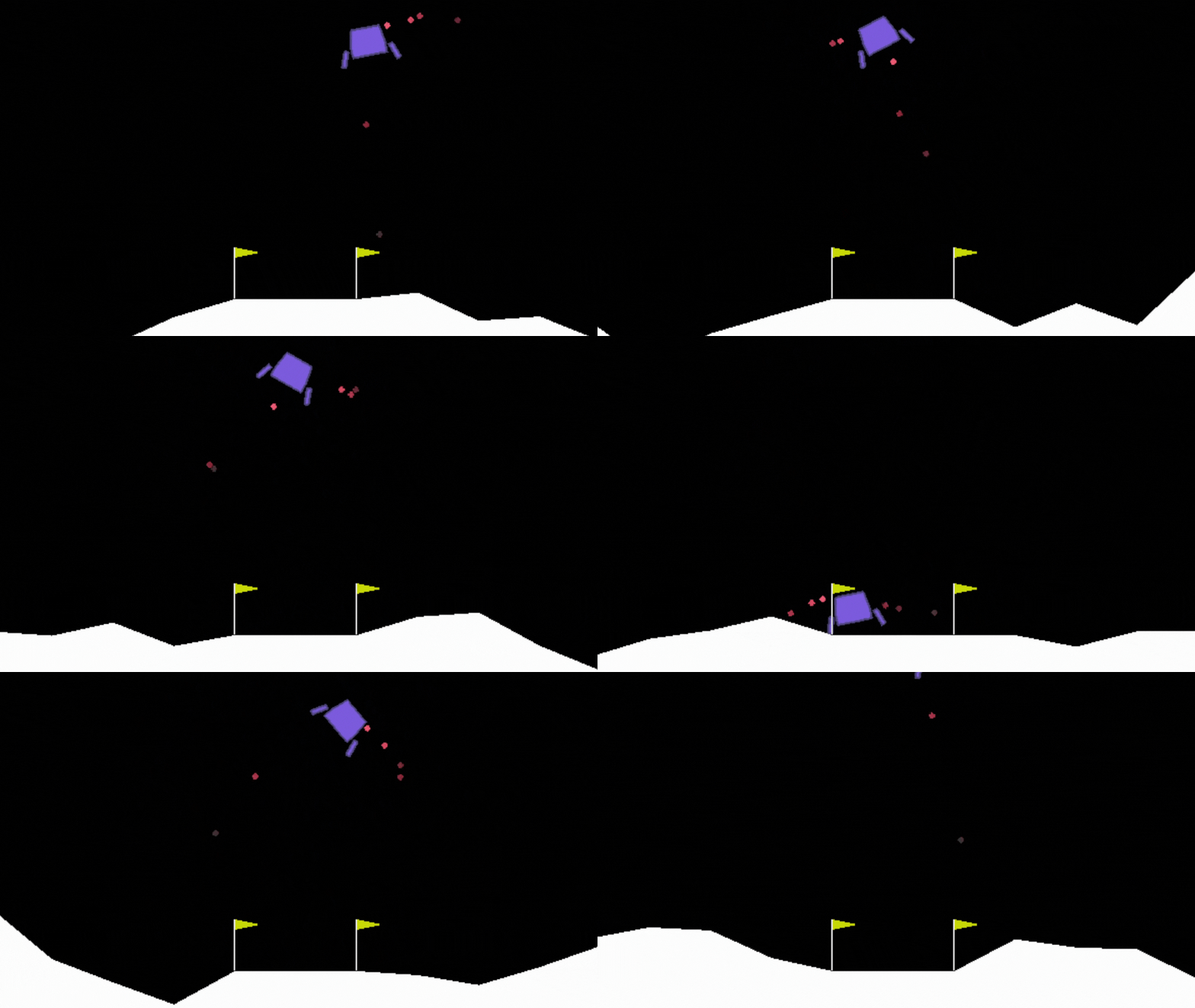
That doesn't look too good, but it's some an agent acting randomly, using env.action_space.sample(). Each time we step in the environment, the step method also returns some information to us. We can collect it with:
obs, reward, done, info = env.step(env.action_space.sample())
Here, we're gathering the observation, reward, whether or not the environment has reported that it's done, and any other extra info. The observation will be those 8 values listed above, the reward is a value reported by the environment, meant to be some sort of signal of how well the agent is accomplishing the desired objective. In the case of the lunar lander, the goal is to land between the two flags. Let's check out the reward and done values:
for step in range(200):
	env.render()
	# take random action
	obs, reward, done, info = env.step(env.action_space.sample())
	print(reward, done)

env.close()
-8.966428059751639 False
-3.2056261702008144 False
-7.918002269808301 False
-5.045565371482126 False
-4.492306794371302 False
-12.056824418777229 False
-8.002752408838138 False
-11.950438693580214 False
-10.814724683236523 False
-4.34849509508271 False
4.965781267653142 False
-5.928775063421142 False
-100 True
-100 True
-100 True
-100 True
-100 True
-100 True
-100 True
As you can see, we got some varying rewards, and then eventually got a bunch of negative -100s and True for the environment being done. This is the environment knowing we crashed.
The objective of reinforcement learning is essentially to keep playing in some environment with the goal of seeking out better and better rewards. So now, we need an algorithm that can solve this environment. This tends to boil down to the action space. Which algorithms can support our action space? What is our action space? It's a single discrete value.
From https://stable-baselines3.readthedocs.io/en/master/guide/algos.html:
Name |
|
|
|
|
Multi Processing |
|---|---|---|---|---|---|
A2C |
✔️ |
✔️ |
✔️ |
✔️ |
✔️ |
DDPG |
✔️ |
❌ |
❌ |
❌ |
✔️ |
DQN |
❌ |
✔️ |
❌ |
❌ |
✔️ |
HER |
✔️ |
✔️ |
❌ |
❌ |
❌ |
PPO |
✔️ |
✔️ |
✔️ |
✔️ |
✔️ |
SAC |
✔️ |
❌ |
❌ |
❌ |
✔️ |
TD3 |
✔️ |
❌ |
❌ |
❌ |
✔️ |
QR-DQN 1 |
❌ |
️ ✔️ |
❌ |
❌ |
✔️ |
TQC 1 |
✔️ |
❌ |
❌ |
❌ |
✔️ |
Maskable PPO 1 |
❌ |
✔️ |
✔️ |
✔️ |
✔️ |
This table gives the algorithms available in SB3, along with the action spaces that they support, along with multi processing. When you have some problem, you can start by consulting this table to see which algorithms you can start off by trying. You should recognize discrete, but then there are things like "MultiDiscrete" and "Box" and "MultiBinary." What are those? Where's continuous?
Box: For now, you can think of this as your continuous space support.
MultiDiscrete: some environments are just one discrete action, but some environments may have multiple discrete actions to take.
MultiBinary: Similar to MultiDiscrete, but for instances where there are only 2 options for each action
It looks like we have quite a few options to try: A2C, DQN, HER, PPO, QRDQN, and maskable PPO. There may be even more algorithpms available later after my writing this, so be sure to check out the SB3 algorithms page later when working on your own problems. Let's try out the first one on the list: A2C. To start, we'll need to import it:
from stable_baselines3 import A2C
Then, after we've defined the environment, we'll define the model to run in this environment, and then have it learn for 10,000 timesteps.
model = A2C('MlpPolicy', env, verbose=1)
model.learn(total_timesteps=10000)
After we've got a trained model, we probably are keen to see it, so let's check out the results:
episodes = 10

for ep in range(episodes):
	obs = env.reset()
	done = False
	while not done:
		# pass observation to model to get predicted action
		action, _states = model.predict(obs)

		# pass action to env and get info back
		obs, rewards, done, info = env.step(action)

		# show the environment on the screen
		env.render()
This is a very simple example, but it's a good starting point. We'll see more examples later. Full code up to this point:
import gym
from stable_baselines3 import A2C

env = gym.make('LunarLander-v2')  # continuous: LunarLanderContinuous-v2
env.reset()

model = A2C('MlpPolicy', env, verbose=1)
model.learn(total_timesteps=10000)

episodes = 10

for ep in range(episodes):
	obs = env.reset()
	done = False
	while not done:
		action, _states = model.predict(obs)
		obs, rewards, done, info = env.step(action)
		env.render()
		print(rewards)
Outputs in the terminal will look something like:
------------------------------------
| rollout/              |          |
|    ep_len_mean        | 190      |
|    ep_rew_mean        | -195     |
| time/                 |          |
|    fps                | 506      |
|    iterations         | 1300     |
|    time_elapsed       | 12       |
|    total_timesteps    | 6500     |
| train/                |          |
|    entropy_loss       | -0.575   |
|    explained_variance | 0.0149   |
|    learning_rate      | 0.0007   |
|    n_updates          | 1299     |
|    policy_loss        | -3.38    |
|    value_loss         | 93       |
------------------------------------
This contains a few statistics like how many steps your model has taken as well as probably the thing you care about most, the episode's reward mean: ep_rew_mean.

Okay, not terrible, but this wasn't enough time apparently to train the agent! Let's try 100,000 steps instead.
import gym
from stable_baselines3 import A2C

env = gym.make('LunarLander-v2')  # continuous: LunarLanderContinuous-v2
env.reset()

model = A2C('MlpPolicy', env, verbose=1)
model.learn(total_timesteps=100000)

episodes = 5

for ep in range(episodes):
	obs = env.reset()
	done = False
	while not done:
		action, _states = model.predict(obs)
		obs, rewards, done, info = env.step(action)
		env.render()
		print(rewards)

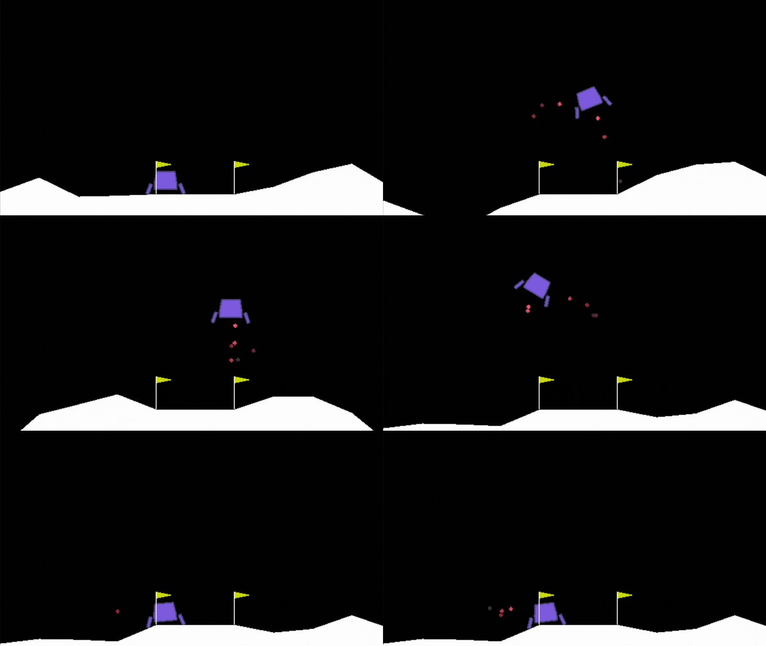
Hmm, well, at least the lander isn't crashing, but it also is pretty rarely actually landing at a reasonable pace. On a realistic problem, you might start thinking about tweaking the reward a bit to maybe disincentivise floating in place, or maybe you just need to be more patient and do more steps. A2C is a fairly old (in terms of reinforcement learning) algorithm, maybe we'll try something else instead? Let's try PPO. We've heard about that one before in the news a few times. To try PPO on our environment, all we need to do is import it:
from stable_baselines3 import PPO
Then change our model from A2C to PPO:
model = PPO('MlpPolicy', env, verbose=1)
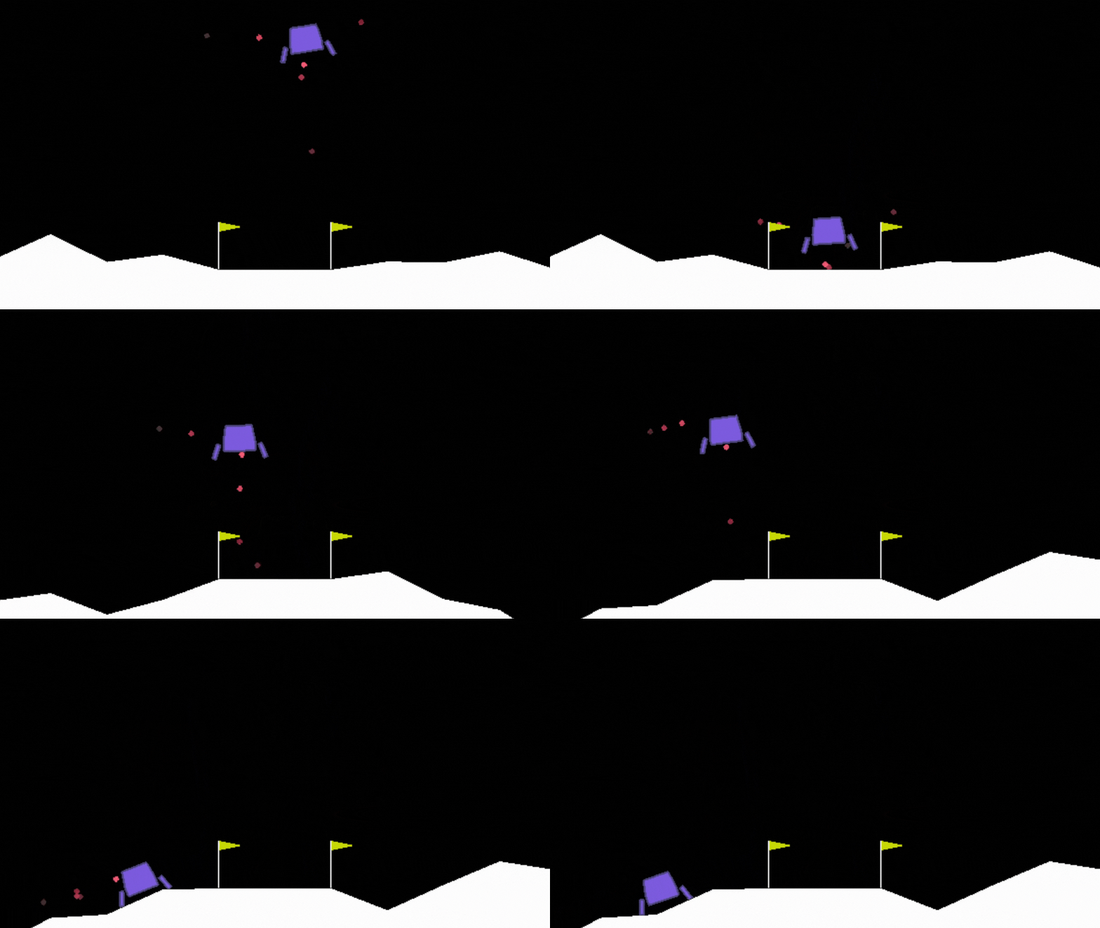
It's that simple to try PPO instead! After 100K steps with PPO:
-----------------------------------------
| rollout/                |             |
|    ep_len_mean          | 575         |
|    ep_rew_mean          | -0.463      |
| time/                   |             |
|    fps                  | 468         |
|    iterations           | 49          |
|    time_elapsed         | 214         |
|    total_timesteps      | 100352      |
| train/                  |             |
|    approx_kl            | 0.013918768 |
|    clip_fraction        | 0.134       |
|    clip_range           | 0.2         |
|    entropy_loss         | -0.92       |
|    explained_variance   | 0.305       |
|    learning_rate        | 0.0003      |
|    loss                 | 73.1        |
|    n_updates            | 480         |
|    policy_gradient_loss | -0.00609    |
|    value_loss           | 76.8        |
-----------------------------------------

I like the looks of this agent much better, and it seems to be better overall.
At this point, you should have a very general idea of how to use Stable Baslines 3 and some of how reinforcement learning works. In the coming tutorials, we'll dive a bit deeper into the various algorithms, action spaces, and much more about using Stable Baselines 3 like tracking our progress, saving and loading models, using custom environments and more.
