Weights and Biases Overview
Deep learning progress tracking and analysis made easy
Have you ever found yourself moving tensorboard logdirs around to other directories for comparisons, maybe sometimes losing them entirely, or forgetting all of the individual settings and details of your model? These are just some of the pain points that the team at Weights and Biases are trying to address.
It turns out the people at Weights and Biases have been trying to get in touch with me since 2019, and Wandb just kind of sounds to me like one of those random popup tech product companies who wants me to advertise their smart wifi enabled spoons, so I just kind of ignored them for a few years. Oops.
After looking into them, and using them quite heavily for the last couple months, I am now a proper addict. Weights and Biases is free to use for personal projects, and you can use it locally as well.
We'll use a very basic example here to just show you how it works, but there are also callbacks to use with other deep learning libraries. For example, I used weights and biases heavily with stable baselines 3 and my reinforcement learning projects.
To get started, you will want to install wandb. Doing this is as simple as:
pip3 install wandb
wandb login
To get your login key, you can head to wandb.ai to create an account. Then go to your settings (https://wandb.ai/settings). In the settings page, you will find your API keys area where you can create a new one or copy an existing one. You will use this key for logging in via your console.
Once that's done, you're ready to rock and roll. Here's a simple mnist deep learning example from the Tensorflow docs:
import tensorflow as tf  # deep learning library. Tensors are just multi-dimensional arrays

mnist = tf.keras.datasets.mnist  # mnist is a dataset of 28x28 images of handwritten digits and their labels
(x_train, y_train),(x_test, y_test) = mnist.load_data()  # unpacks images to x_train/x_test and labels to y_train/y_test

x_train = tf.keras.utils.normalize(x_train, axis=1)  # scales data between 0 and 1
x_test = tf.keras.utils.normalize(x_test, axis=1)  # scales data between 0 and 1

model = tf.keras.models.Sequential()  # a basic feed-forward model
model.add(tf.keras.layers.Flatten())  # takes our 28x28 and makes it 1x784
model.add(tf.keras.layers.Dense(128, activation=tf.nn.relu))  # a simple fully-connected layer, 128 units, relu activation
model.add(tf.keras.layers.Dense(128, activation=tf.nn.relu))  # a simple fully-connected layer, 128 units, relu activation
model.add(tf.keras.layers.Dense(10, activation=tf.nn.softmax))  # our output layer. 10 units for 10 classes. Softmax for probability distribution

model.compile(optimizer='adam',  # Good default optimizer to start with
				loss='sparse_categorical_crossentropy',  # how will we calculate our "error." Neural network aims to minimize loss.
				metrics=['accuracy'])  # what to track

model.fit(x_train, y_train, epochs=3)  # train the model

val_loss, val_acc = model.evaluate(x_test, y_test)  # evaluate the out of sample data with model
print(val_loss)  # model's loss (error)
print(val_acc)  # model's accuracy
I'll be using this for the example, but integrating just about any script is very simple.
We essentially just need to to 3 things. First, we'll import wandb and the WandbCallback:
import wandb
from wandb.keras import WandbCallback
Next, we need to initialize wandb with a project name:
wandb.init(project="WandB tutorial")
Third, when we run model.fit, we'll add the WandbCallback to the callbacks:
model.fit(x_train, y_train, epochs=3, callbacks=[WandbCallback()])
That's all there is to it for basic tracking! Let's run this and check out the results in Wandb. Full code:
import tensorflow as tf  # deep learning library. Tensors are just multi-dimensional arrays

# adding this:
import wandb
from wandb.keras import WandbCallback

wandb.init(project="WandB tutorial")

mnist = tf.keras.datasets.mnist  # mnist is a dataset of 28x28 images of handwritten digits and their labels
(x_train, y_train),(x_test, y_test) = mnist.load_data()  # unpacks images to x_train/x_test and labels to y_train/y_test

x_train = tf.keras.utils.normalize(x_train, axis=1)  # scales data between 0 and 1
x_test = tf.keras.utils.normalize(x_test, axis=1)  # scales data between 0 and 1

model = tf.keras.models.Sequential()  # a basic feed-forward model
model.add(tf.keras.layers.Flatten())  # takes our 28x28 and makes it 1x784
model.add(tf.keras.layers.Dense(128, activation=tf.nn.relu))  # a simple fully-connected layer, 128 units, relu activation
model.add(tf.keras.layers.Dense(128, activation=tf.nn.relu))  # a simple fully-connected layer, 128 units, relu activation
model.add(tf.keras.layers.Dense(10, activation=tf.nn.softmax))  # our output layer. 10 units for 10 classes. Softmax for probability distribution

model.compile(optimizer='adam',  # Good default optimizer to start with
				loss='sparse_categorical_crossentropy',  # how will we calculate our "error." Neural network aims to minimize loss.
				metrics=['accuracy'])  # what to track

# adding the WandbCallback
model.fit(x_train, y_train, epochs=3, callbacks=[WandbCallback()])  # train the model

val_loss, val_acc = model.evaluate(x_test, y_test)  # evaluate the out of sample data with model
print(val_loss)  # model's loss (error)
print(val_acc)  # model's accuracy
While running (or when it's done), head over to wandb.ai/YOURNAME/projects to see hopefully the project and click on it. You should see something like:
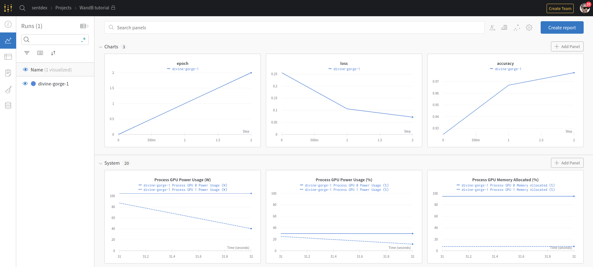
This is your project overview page, showing all of your runs for the project. For now we just have the one, but this is where you might compare many different models. Each of the graphs can be customized, you can add new ones, move them around and change things like the axis to be step or relative or wall time...etc. Since we didn't specify any name, wandb generated a random name for the run for us. It can be tempting to put various settings and parameter info in the name of the run, if you're like me you've probably done that with your tensorboard runs, but that's not necessary here. Click on the run, and this will take you to the run's page. Immediately, we can go to the overview tab and see a bunch of information, like when this run happened, the system hardware it was run on, and even the command that was used to run it. Under system, we can review system utilization, and things like running temperatures. We can check out the model itself, in case we forgot the parameters, we can check logs, which is a console log of all of the running, and there are some files too. If your model used tensorboard and you wanted to sync that too, that'd be here, I'll show that in a bit. Anyway, tons of information here, almost all of which are things I've historically needed to go back and check for, but you don't even need to think about it, it's all here.
Sometimes, however, you want to maybe track a bit more, maybe more of your hyperparameters, and this is where you probably historically would have stuffed them into your tensorboard log name. Here are some examples of hyperparameters that you might use:
import os

os.environ["CUDA_VISIBLE_DEVICES"] = "0"
HM_GPU = 1
MACHINE = "Puget"
GPU = "3090"
NVLINK = "Yes"
We can then add a config dictionary for wandb:
conf_dict = {"GPU":GPU,
				"Machine":MACHINE,
				"HM_GPU":HM_GPU,
				"NVLINK": NVLINK,
}
Then the wandb init method becomes something more like:
wandb.init(
	project=f'WandB tutorial',
	entity="sentdex",
	config=conf_dict,
	#sync_tensorboard=True,  # see if it works ig
	name=f'{MACHINE}-{GPU}-{HM_GPU}GPU'
	)
The config dictionary is where you can save all of the hyperparameters that you might think you'll want, and then the name parameter in the wandb init method allows you to set the name to something you want, rather than it just being totally random. Running this again, we can check out the results. It should look very similar in the project overview. Click on the run itself next, then overview, and then you should see a config area that looks like:
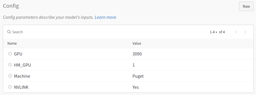
This is where you can further store various information about the model. You can also write notes:

So, just in general, wandb is just plain nice for experiment tracking, especially if you're running many models and tests, or you're running them over a long period of time, or if you're running them on various distributed machines...etc.
Next, I'd like to show some actual examples of my uses with WandB. I am by no means a poweruser, nor do I know or use all of the features, but some of the things here are pretty cool. For example, if you have a lot of runs in a project, there's the table tab you can view:
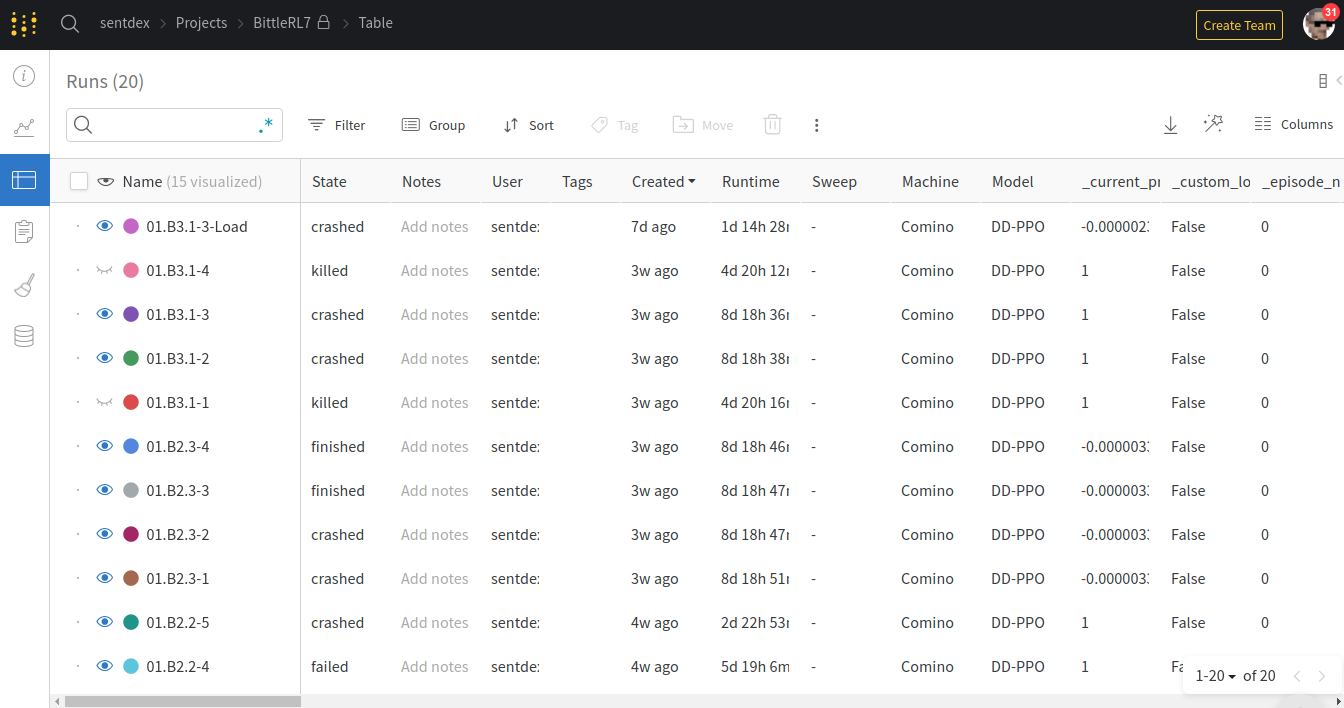
On this table, you can move around columns and sort them as desired. One common thing might be to sort by loss, accuracy, or, in the case of reinforcement learning, reward.
In this case, we're looking at a few of the reinforcement learning with Stable Baselines 3 runs, where I am training a robot dog walk in a simulator. Stable Baselines 3 for example is one of the other deep learning libraries that has a callback already made for it for weights and biases, which again makes it as easy as converting the script shown above.
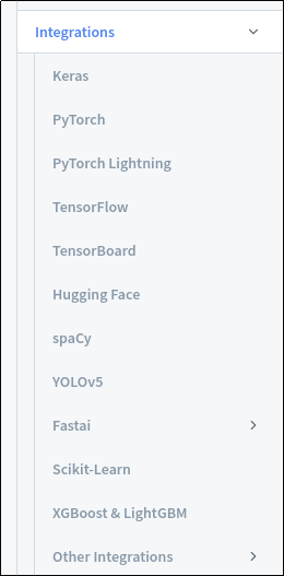
If you're looking to integrate into Pytorch, or other libraries, you can check out the WandB + Pytorch docs. It's equally simple, and there are many others:
Beyond this, we can also see more of the performance tracking:
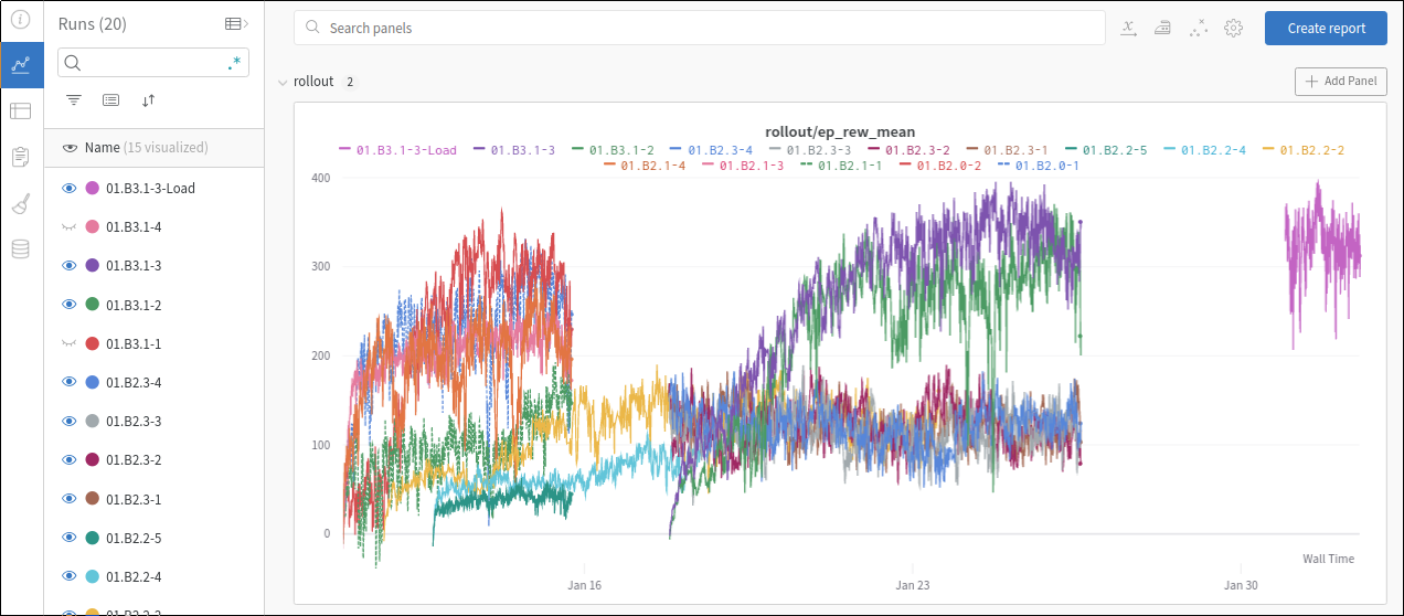
All charts can be customized, you can add more like line or bar charts. You can make your line charts with an X axis of step, wall time, or relative time.
And, again, all these runs are tracking the performance, along with all of the hyperparameters, the system it was trained on, the system performances for CPU and GPUs, and more. It's all stored and logged here, should you need it.
-
Wandb.ai - Tracking and R&D for your deep learning models in Python